
As of July 20, 2026, anyone can download calibrated radar products from the NASA-ISRO Synthetic Aperture Radar mission. One early frame shows Nunatak Zaterjavshijsja in East Antarctica as a green-and-magenta hummingbird carved by glacier stress.
The image is more than a viral curiosity. It marks the start of an open, near-global time series that peers through snow and ice every 12 days.
The Hummingbird Hidden in the Ice
The rocky peak rises at center-left while a glacier flows northeast toward the ocean. Stress around the obstruction fractures the ice into deep crevasses. In the false-color product those cracks appear as sharp green lines; smoother ice surfaces register magenta; zones of mixed scattering turn white.
Seongsu Jeong, the JPL signal analysis engineer who produced the frame, said: “First, it’s a beautiful image, with rich details of features that provide insights to how the glacier is moving. Then, because radar can often see through snow and deep into the ice, NISAR can observe fundamentally different properties of Antarctic ice than can be seen in optical imagery. With NISAR we’re seeing what’s hidden beneath the surface.”
The same landscape in optical light from Landsat 9 is almost pure white. Only faint shadows hint at the mountain. The L-band image of the Antarctic nunatak was collected in August 2025 during system tests and released with the public data stream.
That contrast is the point. Optical sensors record sunlight bouncing off the top of the snow. Radar records how the ice itself scatters energy that has already traveled some distance into the pack. The hummingbird shape is simply the first pattern many viewers recognized; the science value is the subsurface structure the colors encode.
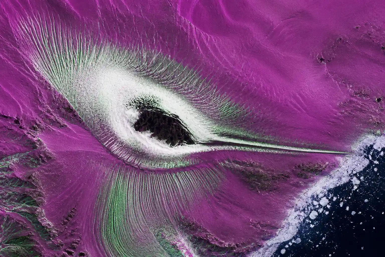
What the Colors Reveal About Scattering
NISAR transmits horizontally polarized microwaves. The polarization of the return tells scientists what the surface did to the signal.
| Color | Scattering type | Typical surface |
|---|---|---|
| Magenta | Surface (horizontal return) | Smooth ice |
| Green | Volume (vertical or cross-pol) | Crevasse walls, snow pack |
| White | Strong mixed return | Combined surface + volume |
L-band operates at a 24 cm wavelength. That length lets energy penetrate snow and, under the right conditions, ice. Optical cameras stop at the top surface.
When a crevasse wall faces the radar, energy bounces back with a vertical component and paints green. When the ice is smooth and level, the return stays horizontal and paints magenta. Mixed zones light up white because both mechanisms operate at once. The palette is therefore a map of physical process, not an artistic choice.
Two Radars on One Platform
NISAR is the first free-flying satellite to fly both L-band and S-band synthetic aperture radars. The longer L-band wavelength reaches the ground under forest canopies and probes ice structure. The shorter S-band wavelength is more sensitive to vegetation canopies and certain ice-surface details.
- L-band: global coverage, ~240 km swath, along-track resolution about 7 m, cross-track 2 to 8 m depending on mode
- S-band: focused on India and selected science targets including polar ice, complementary polarimetry
- 12-day exact-repeat orbit at 747 km altitude
- Left-looking geometry that gives complete Antarctic coverage at the cost of a small Arctic gap
- 12-meter (39-foot) deployable radar reflector, the largest NASA has flown for this purpose
Together the pair builds denser observations of ecosystems, ground deformation, and cryosphere change than either band alone. Mission documentation lists the 240 km swath and 2-to-8 m resolution as core design goals.
The shared 12-meter reflector feeds both radars. That common aperture keeps the two wavelengths geometrically aligned, so dual-frequency products can be formed without large co-registration offsets. Researchers can therefore treat the pair as a single instrument rather than two separate missions that happen to share an orbit.
Where the Files Live and How to Get Them
Calibrated L-band products covering acquisitions from June 17, 2026 onward began flowing July 20 through the Alaska Satellite Facility DAAC and NASA Earthdata Search. Users can also pull them via ASF Vertex, APIs, or the asf_search Python package. The mission generates dozens of terabytes of science data every day.
Earlier limited releases included roughly 25 sample products in January 2026 and more than 100,000 pre-calibrated files in February. Full earlier science-operation data is scheduled for release by the end of 2026. On the Indian side, S-band products on the Bhoonidhi portal started with Cycle 25 (from July 8, 2026) and will expand with reprocessed historical scenes.
All products follow a free and open data policy. The calibrated L-band products now at ASF DAAC sit alongside decades of earlier SAR archives, letting researchers stack long time series immediately.
The open policy removes the usual lag between acquisition and analysis. A graduate student or a national ice center can pull the same calibrated granules on the same day and begin interferometric processing without waiting for a proprietary release window.
Why Antarctica Gets Special Treatment
The left-looking design was chosen in part so NISAR can map nearly the entire Antarctic ice sheet. Optical satellites struggle with polar night, clouds, and the featureless white surface. Radar works day or night and through cloud, and L-band adds subsurface information.
Crevasse fields, ice velocity, and grounding-line changes become measurable with the same 12-day cadence used over forests and cities. That cadence matters for short-term ice dynamics that feed into sea-level projections. Related work on Antarctic ice and Southern Ocean carbon links already shows how surface change couples to broader climate systems.
Public reaction on X treated the hummingbird shape as delightful pareidolia, yet the same posts repeatedly noted that ordinary cameras would have shown only white. The high-engagement NASA Earth and JPL posts drove traffic straight to the open archive.
Because the orbit geometry favors the south, Antarctica receives wall-to-wall coverage that the Arctic does not fully share. That trade-off was deliberate: the densest radar record is being built first where optical data are scarcest and where ice-sheet mass loss carries the largest sea-level consequence.
What Researchers Can Do First
The science objectives target four domains: solid-Earth deformation (earthquakes, volcanoes, landslides, subsidence), ecosystem carbon stocks, ice-sheet and sea-ice response to climate, and soil-moisture patterns. Early examples already include Mexico City subsidence maps, Venezuelan earthquake displacement, agricultural growing-season change, and the Antarctic crevasse fields.
Because both ascending and descending passes are collected, interferometric pairs form quickly. Pixel-offset and unwrapped-interferogram products support velocity and deformation studies without waiting years for a new mission. Forest biomass and wetland inundation also benefit from the dual-frequency combination.
The NISAR mission science objectives were set by the 2007 Decadal Survey and refined through more than a decade of joint NASA-ISRO work. The satellite itself rode a GSLV-F16 from Satish Dhawan Space Centre on the July 30 2025 joint launch from India. Science operations began in January 2026 after commissioning.
- Solid-Earth: rapid deformation maps after earthquakes or during volcanic unrest
- Ecosystems: dual-band sensitivity to canopy structure and biomass
- Cryosphere: 12-day ice velocity and crevasse evolution
- Hydrology: soil-moisture and inundation patterns across seasons
Those four threads share the same calibrated archive, so a researcher studying Mexico City subsidence can reuse processing scripts later on Antarctic grounding lines without rebuilding the entire pipeline.
How the Mission Timeline Unfolded
The path from launch to open calibrated products followed a clear sequence of milestones already on the public record.
- July 30, 2025 – GSLV-F16 lifts NISAR from Satish Dhawan Space Centre.
- August 2025 – System-test L-band image of the Antarctic nunatak is acquired.
- January 2026 – Science operations begin; roughly 25 sample products released.
- February 2026 – More than 100,000 pre-calibrated files become available.
- June 17, 2026 – Start of the acquisition window for the first calibrated L-band stream.
- July 8, 2026 – S-band Cycle 25 products appear on the Bhoonidhi portal.
- July 20, 2026 – Calibrated L-band products open to the public at ASF DAAC.
Full earlier science-operation data is scheduled for release by the end of 2026. Continuous forward processing then keeps the archive current with every new 12-day cycle.
The compressed schedule matters because interferometry thrives on dense temporal sampling. Each successive release shortens the gap between first light and usable time series, letting change-detection studies start while the mission is still young.
Why Dual Frequency Changes the Picture
Single-band SAR missions force a choice: longer wavelengths for penetration or shorter wavelengths for fine surface detail. NISAR removes that trade-off by carrying both.
| Band | Strength | Primary targets |
|---|---|---|
| L-band | Penetration through canopy and snow | Ground deformation, ice structure, soil moisture |
| S-band | Sensitivity to canopy and ice-surface texture | Vegetation, selected polar ice details |
Over forests the L-band return reaches the ground while the S-band return interacts more with leaves and branches. Over ice the same pairing separates volume scattering inside the pack from surface roughness at the top. The result is a richer scattering signature than either wavelength can supply alone.
Because the two radars share the identical 12-day orbit and left-looking geometry, their observations are naturally co-located. Analysts can form dual-frequency products without the geometric compromises that arise when data from separate satellites must be forced into a common grid.
The Archive Will Only Grow
By late 2026 the full first-year science record should sit in the public archive. Continuous forward processing means every new 12-day cycle adds another global layer. Dozens of terabytes per day will accumulate into one of the densest radar records of Earth’s land and ice ever assembled.
Coverage runs from a few degrees of the South Pole to 77.5 degrees north. Cities, farmland, glaciers, and wetlands all receive the same systematic attention. The hummingbird image is simply the first frame many people noticed. The lasting product is the open time series behind it.
As the stack thickens, seasonal and multi-year signals become separable from short-term noise. That depth is what turns a striking single image into a climate and hazards observing system that any researcher can query.
Frequently Asked Questions
What does NISAR stand for and who built it?
NISAR is the NASA-ISRO Synthetic Aperture Radar, a joint Earth-observing satellite. NASA/JPL supplied the L-band radar and 12-meter reflector; ISRO supplied the spacecraft bus and S-band radar. It launched July 30, 2025 from India’s Satish Dhawan Space Centre.
How often does NISAR image the same place?
The satellite repeats its ground track every 12 days, collecting both ascending and descending passes over nearly all land and ice surfaces. That cadence supports continuous interferometry and change detection without long gaps.
Why can the radar see through snow and ice when cameras cannot?
L-band microwaves at 24 cm wavelength penetrate dry snow and, under suitable conditions, ice. They also pass through cloud and operate in darkness. Optical sensors measure only reflected sunlight from the top surface.
Where can anyone download the free data?
L-band products are available through the Alaska Satellite Facility DAAC, NASA Earthdata Search, Vertex, APIs, and the asf_search package. S-band products are released on ISRO’s Bhoonidhi portal. No fees or special licenses are required for scientific or educational use.
What makes the dual-frequency design unique?
NISAR is the first free-flying satellite to carry both L-band and S-band SARs. The two wavelengths respond differently to vegetation structure, soil moisture, and ice properties, giving a more complete picture than single-band systems.